^{(Last updated: 08/30/2019 | PDF | PERSONAL OPINION)}

Yes, you guessed it right! We’re going to look at solving traditional analytic problems with technologies behind deep learning. In this broader context, the term “deep” is too limiting as the computation flow may takes any shape from a list of components stacked together (deep) to hierarchical (tree) to spaghetti (graph). And the term “learning” is intentionally misleading as solutions are reached with mechanic (dumb) maneuvers without understanding.

From Control Theory to Deep Learning

When I was struggling though my Advanced Automatic Control Theory class, I was wondering when I would ever get to use these stuffs. Well, now that I’m talking about deep learning, I can’t start without mentioning feedback control, the mechanism that gave birth to the whole industrial revolution, and now powering the AI revolution, and, if you indulge with me, how those billions of neurons might actually work in human brain.

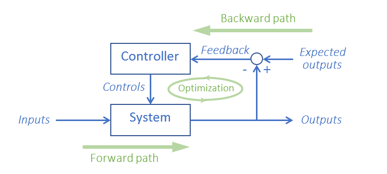
Feedback control is ignorant, which is rightfully touted as a virtue in the control theory circle: “feedback control system is easy to implement, because it requires no knowledge of the source or nature of the control parameters, nor does it require much information about how the system itself works. Feedback control action is entirely empirical (a.k.a. numerical, computational).”

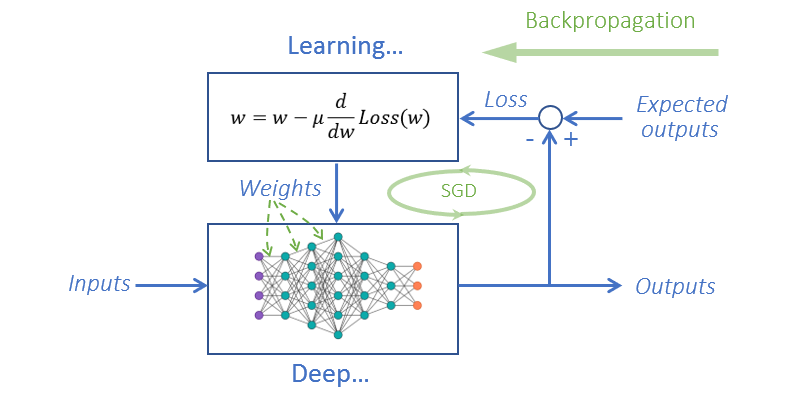
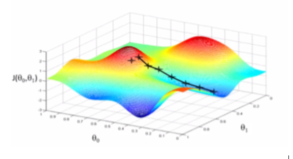
Using one of the gradient based nonlinear optimizer such as stochastic gradient descent(SGD) to do the “Optimization”, renaming “Feedback” as “Loss” and the backward path as “backpropagation”, labeling your system as “deep” and marketing the mechanic updates of gradients as “learning”, you got what everybody is talking nowadays: deep learning!

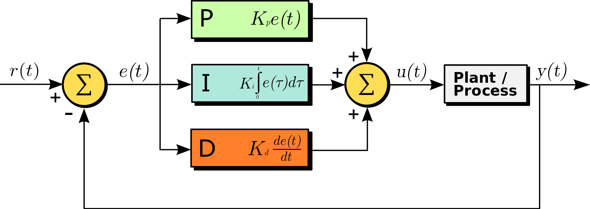
Deep learning only uses the “D” part of the most widely used PID controller. To the deep learning developers here at SAS, finding ways to incorporate integral and proportional components in the optimizer might put us ahead of the AI competition. In below block diagram of a PID controller in a feedback loop, y(t) is the measured outputs and r(t) is the expected outputs.

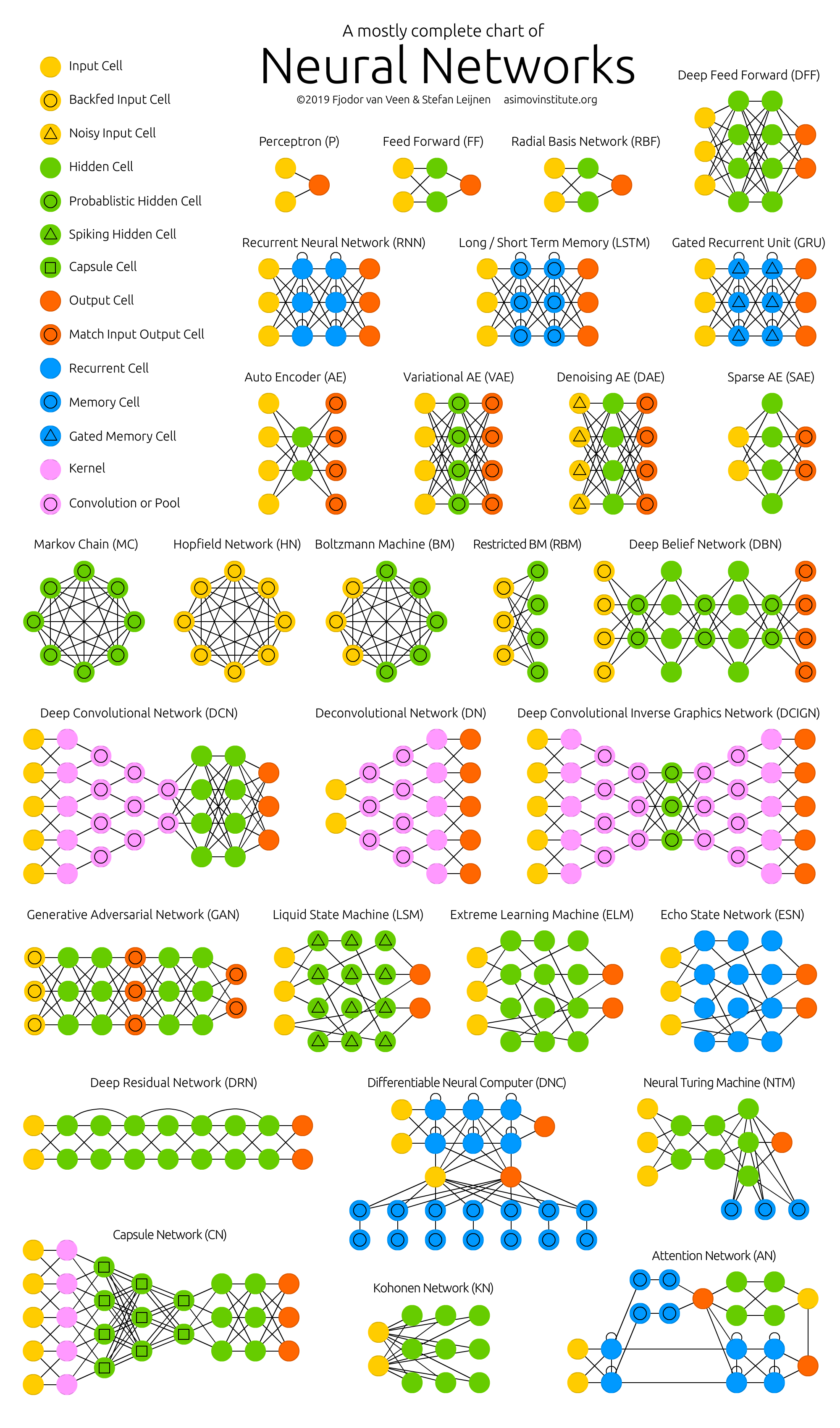
To be fair, deep learning folks’ contributions lie in those ingenious architectures, the specific intricate arrangements of the specially purposed computational components (ReLU, pooling, embedding…), enabling their system to exhibit intelligent behaviors indistinguishable from or even better than that of human. By and large, deep learning architecture design is a try-and-error art, rather than science (think alchemists vs chemists). This is evident from the designer names attached to popular architectures: LeNet, AlexNet, ZF Net, GoogleLeNet… Therefore, the competitive advantage of AI lies in architecture design. We may reimplement existing architectures or resolve problems that are better solved by others all day, only when we come up with our own branded architecture such as SasOR_MIP_NET or ViyaFcstNet for problems others haven’t looked at, we’re in the league of leaders of AI.

What TensorFlow Really Is

If you associate TensorFlow with only cat pictures and deep learning, I don’t blame you, but you’re missing the forest for the trees. From their official self-description of “end-to-end open source platform for machine learning”, even the TensorFlow people don’t realize its true potential.

TensorFlow is a platform to develop and deploy any software-implemented system that can be modeled with differentiable programming. You only need to tell TensorFlow three aspects of your system:

What are the control parameters of your system (controls, knobs)?
How to compute outputs from inputs (the forward path)?
How to compute loss from computed and expected outputs (the feedback)?

TensorFlow will figure out (via the backward path) and tell you the optimized values of the control parameters, which is effectively the structure of your system. TensorFlow does it by minimizing the loss function w.r.t. the control parameters, with one of the gradients based non-linear optimization algorithm.

Differentiable Programming

TensorFlow is a programming language with which you describe how your system works and a tool chain which automates away the differentiation and optimization of your program. The way you tell TensorFlow about your system is encoding your system structure in programming statements that is continuous and differentiable.

Let’s start with a simple system y = x^2, which we all know is continuous and differentiable with y’=2x. You set x to 1.0 and ask TensorFlow what the gradient of y w.r.t. x at that point, you get 2.0!

x = tf.Variable([[1.0]])
with tf.GradientTape() as tape:
  y = x * x

grad = tape.gradient(y, x)
print(grad)  

# => 2.0

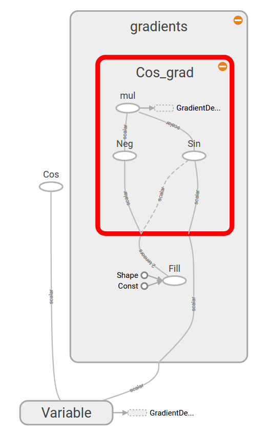
For another example, let’s look at a system y=cos(x) where y is the output and the loss, and x are both the input and the only control parameter.

x = tf.Variable(initial_value=3.0) /* control parameter */
y = tf.cos(x)                      /* x => y */  
tf.train.GradientDescentOptimizer(learning_rate=0.01).minimize(y)

If you look at the compute graph generated by TensorFlow, you’ll notice alongside the branches corresponding to your system y=cos(x), TensorFlow figures out how to compute gradients for your system: y’ = -sin(x)!

Automatic differentiation is the technique that does the magic and not only the cos() function is differentiable, matrix multiplication, conditionals, loops, branches and recursions are all amenable to autograd , giving you expressive power to model your system.

As you can see by now, once your system is modeled with differentiable programing statements, you can delegate the search for the optimal system structure to TensorFlow.

Linear Regression the Differentiable Programming Way

With slope (beta1) and intercept (beta0) as the control parameters and mean squared error as loss function, we may solve the linear regression problem with a gradient descent optimizer.

# Inputs
X = tf.placeholder("float") 
Y = tf.placeholder("float") 

# What are the control Parameters ?
beta1 = tf.Variable(0.3, dtype = tf.float32, name = "beta1") 
beta0 = tf.Variable(0.0, dtype = tf.float32, name = "beta0") 

# How to compute outputs from inputs?
y_pred = tf.add(tf.multiply(X, beta1), beta0) 

# How to compute loss function from outputs and expected
#  outputs? Mean Squared Error (MSE)
loss = tf.reduce_sum(tf.pow((y_pred - Y), 2)) / (2*n)

# Optimizer
optimizer = tf.train.GradientDescentOptimizer(0.01).minimize(loss) 
  
# Global Variables Initializer
init = tf.global_variables_initializer() 

# Tensorflow Session
with tf.Session() as sess: 
    # Initializing the Variables
    sess.run(init) 

    # Iterating through all the epochs 
    for epoch in range(100): 
        # Feeding data into the optimizer using Feed Dictionary 
        for (_x, _y) in zip(px, py): 
            sess.run(optimizer, feed_dict = {X : _x, Y : _y}) 
          
    # Retrieve values for use outside the Session 
    loss_val = sess.run(loss, feed_dict ={X: px, Y: py}) 
    weight   = sess.run(beta1) 
    bias     = sess.run(beta0) 
    
    # Calculate the predictions 
    predictions = weight * px + bias

Linear Regression the Theoretical Way

We all know for simple linear regression there is the theoretical optimal parameter estimates which involves only matrix operations. Complete with a linear algebra package, TensorFlow can be used as IML to solve linear regression algebraically:

    ones = np.ones(n)
    X_matrix = np.matrix(np.column_stack((px, ones)))
    Y_matrix = np.transpose(np.matrix(py))

    X_tensor   = tf.constant(X_matrix)
    Y_tensor   = tf.constant(Y_matrix)
    XtX_tensor = tf.matmul(tf.transpose(X_tensor), X_tensor)
    XtY_tensor = tf.matmul(tf.transpose(X_tensor), Y_tensor)

    sol = tf.matmul(tf.matrix_inverse(XtX_tensor), XtY_tensor)
    soln_opt = sess.run(sol).tolist()
    weight_opt, bias_opt = soln_opt

    # Calculating the predictions 
    predictions_opt = weight_opt * px + bias_opt 
    sess.run(beta1.assign(weight_opt[0]))
    sess.run(beta0.assign(bias_opt[0]))
    loss_opt = sess.run(loss, feed_dict ={X: px, Y: py})

Probabilistic Programming

It’s fair to say deep learning in specific and differentiable programming in general knows no math, because if you can express the forward path and loss function of your system with programming statements (not much math), frameworks like TensorFlow automatically (with lots of math) finds the solution for you. This “for dummy” approach enables data analysts and even high schoolers to build AI models by brute force. A data scientist may come up with the perfect loss function quickly, but data analysts and high schoolers alike can eventually get there by try and error.

Is there a “for dummy” approach for people who knows and can model prior knowledge of their system with college level math? Enter probabilistic programming.

The probabilistic approach of problem-solving starts with modeling the uncertainty of a system with a joint probabilistic distribution on variables whose values are known (observed) and variables/parameters whose values are typically unknown (latent). Also known as the generative model, the joint distribution is normally constructed bottom up from proposal (prior) distributions of observed and latent variables. The solution of the system is reached by inference tasks such as parameter finding for posterior distributions or expected values calculation of various statistics on conditional distributions. Again, a probabilistic programming system enables probabilistic modeling of your system with programming statements and automates away the math and computational heavy inference tasks for you.

With probabilistic programming system all you need to do is:

Provide proposal distributions for the parameters (latent variables) of your system.
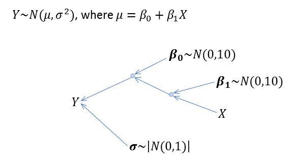
Construct the joint distribution of the observed target variable (Y) in terms of the latent parameters (β) and the observed input variables (X).

The probabilistic programming system will automatically infer the marginal distributions of the parameters conditioned on the observed input and target variables. Monte Carlo simulation or variational optimization, you don’t need to care the math behind and implementation details of the inference engine.

Linear Regression the Probabilistic Programming Way

It’s only natural for us to resolve our simple linear regression problem again, with probabilistic programming approach. As taught in every regression class, we assume Y to be normally distributed with an unknown variance, which is normally distributed itself. We also assume the slope and intercept of the regression line follows a normal distribution.

Below Python program encode our assumptions into programming statements:

import pymc3 as pm 
with pm.Model() as model: 
    # Define prior distributions of parameters
    beta0 = pm.Normal('beta0', 0, sigma=20)
    beta1 = pm.Normal('beta1', 0, sigma=20)
    sigma = pm.HalfCauchy('sigma', beta=10, testval=1.)

    # Define likelihood (sampling joint distribution)
    jointDist = pm.Normal('Y', mu = beta0 + beta1 * px, sigma=sigma, observed = py)

    # Inference! 
    start = pm.find_MAP(model=model)
    step  = pm.Metropolis()     
    trace = pm.sample(1000, step=step) 

estimate = pm.summary(trace)
predictions_pp = estimate.at['beta0','mean'] + estimate.at['beta1','mean'] * px  
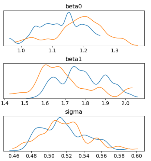
pm.traceplot(trace)

In the inference phase, we take samples from the proposal parameter distributions (orange in below graph), accept or reject the proposal based on observed data. The result is a posterior distribution (blue) of our parameters with the peak being the optimal parameter estimates. Better yet, we got the uncertainty of those parameter estimates for free!

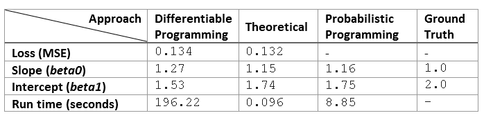
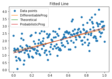
Which Way is Better?

Theoretical approach produces the optimal solution, but it takes a master or Ph.D. level data scientist who understand the math to program it. On the other hand, the differentiable and probabilistic programming way requires only rudimentary math. Also let’s not forget, for those problems that are too complex to tackle theoretically, the differentiable and probabilistic programming way maybe the only practical way.

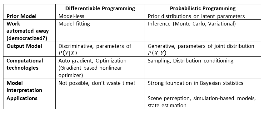
Differentiable vs Probabilistic Programming

With two styles of programming solving the largely overlapping problems, a comparative study of the two follows:

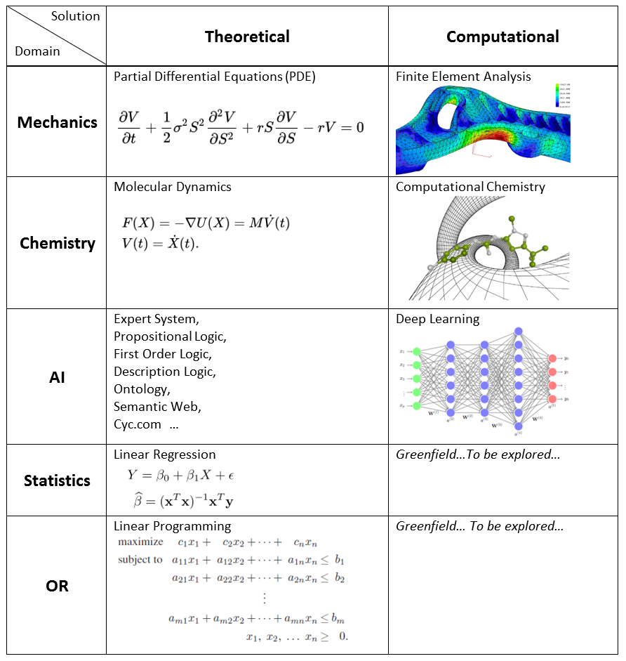
Computational Approach to Problem Solving

When it’s too complex or expensive to understand and solve a problem theoretically, we resolve to solutions obtained by computational approaches. The history of science and mathematics has seen this pattern again and again, in mechanics, fluid dynamics, chemistry, finance, and recently AI. Almost all computational approaches can be thought of as simulation: following basic principles of the problem domain, evolve the solution by heuristics (divide and conquer, GRASP, SGD…) until stopping criterion (epoch, epsilon…) is met. Differentiable and probabilistic programming are such computational approaches.

Damn, West Coast Folks are Already on It

Just as I thought I discovered a new world where we can be the first mover, news came that Google and Amazon are already applying deep learning techniques to statistical and forecasting problems. Given their histories of developing new then open sourcing/publishing old technologies, they must have used them for quite a long time in their business operations.

TensorFlow Probability (TFP) from Google, which is a Python library built on TensorFlow that makes it easy to combine probabilistic models and deep learning on modern hardware (TPU, GPU). TFP offered probabilistic programming on top of differentiable programming that comes with TensorFLow.
GluonTS from Amazon, which is a library for deep-learning-based time series modeling.
Prophet from Facebook, which is a forecasting library based on probabilistic programming. A modeless computational approach by nature, it “(produce) a reasonable forecast on messy data with no manual effort. … is robust to outliers, missing data, and dramatic changes in your time series”.

Please don’t laugh at their lack of theoretical and practical knowledge in the analytics domains that we excel. Their superior command of the computational technologies may soon render domain specific theory and knowledge unnecessary to obtain good enough solutions. To maintain the leader position, we must humbly learn about the computational technologies from them and combine our deep domain knowledge with computational approaches in our solution.

Summary

For analytics problems or part of the problem that are theoretically intractable, we could exploit the computational techniques behind deep learning: Differentiable Programming. Together with probabilistic programming (simulate the task and see what happens), we have two ways of getting a solution to a problem without having to analyze it mathematically.

With objective function being the first piece of any optimization problem model, Operations Research (OR) is a natural fit to benefit from the deep learning paradigm. But I’m not in the position to say whether the constraints of OR problems break the “continuous and differentiable” requirement of differentiable programming. The point is, for the traditional analytics folks, there is this thing from neighboring AI community that can help to solve your problems!

There you have it, differential and probabilistic programming, the forest behind the specimen tree called “deep learning”. Ten years from now when you look back at the stage of AI as is now, you’ll see that computer vision and NLP are just two small fish AI can catch. Differentiable and probabilistic programming are the way of fishing to catch them and other bigger fish in the days ahead!

References:

The complete TensorFlow program for our example problems. No TensorFlow? No problem. Google CoLab is an online playground for TensorFlow.
Differentiable programming in Yann LeCun’s own words.
The origin of the term “differentiable programming”
A must read for auto-grad, Automatic Differentiation in Machine Learning: a Survey.
On Machine Learning and Programming Languages, by folks behind Julia. Flux is the differentiable programming language they designed from scratch.
Differentiable programming (Deep learning) has been used to solve problems in jet physics, PDE’s, robotics and many more.
A more realistic linear regression example from official TensorFlow documentation.
I’m still in the process of wrapping my mind around TensorFlow’s probabilistic programming offering, Linear regression with TensorFlow Probability.
Probabilistic models of cognition explores the probabilistic approach to cognitive science.
MIT has a dedicated Probabilistic Computing Project.
A two pager worth reading: The principles and practice of probabilistic programming.
The background section of this paper has the most succinct description of the field of probabilistic modeling and inference.
Our probabilistic linear regression example follows closely to steps in Probabilistic programming in Python using PyMC3.
Variational Inference: A Review for Statisticians.
Differences between Discriminative vs Generative models.
A Hacker News discussion on what companies are using probabilistic programming.
The invention of NUTS (No-U-Turned-Samplers) enabled probabilistic programming approach.
Deep Learning, a critical appraisal
Time Series prediction, a short introduction for pragmatists. Valuable discussion on forecasting, especially the book “Deep learning for time series forecasting”.

Deep Statistics

Dr. Mindle's Musings