(Last updated: 12/12/2019 | PDF | PERSONAL OPINION)
“Open” is a virtue made from the reality that no single analytics vendor has everything customer want and the need to get things done by maneuvering two or more tools simultaneously. If you expect a carpenter to use only BLACK+DECKER tools, no matter how complete your product line is, you’ll be disappointed.
Openness resides at different levels of the analytics platform stack, it has directions, and it may take different styles of integration. Software that is open doesn’t have to be open sourced.
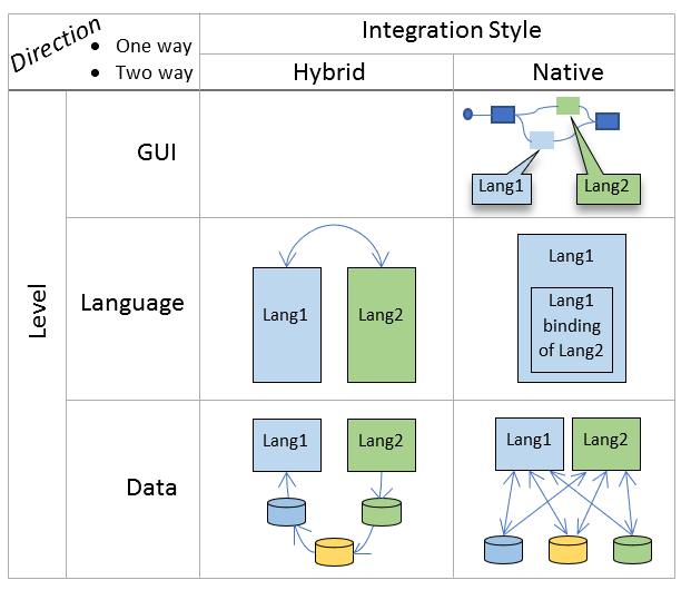
Language Level Hybrid Integration
Mixing different programming languages together in one program has been done through and though. However, they’re done almost always out of desperation. When Python is intolerably slow, you turn the compute intensive part into a C function and call it from within the Python program. When C is too slow? You call into assembly language from within the C program. The context switching and handshaking between different languages are so counterproductive that the hybrid approach should be avoided as much as possible.
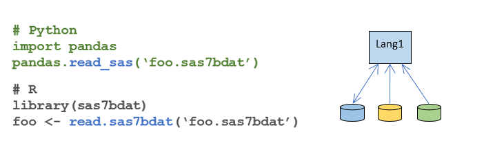
To use a piece of compute written in Lang2 within Lang1, you’d interleave the two languages together as shown below:
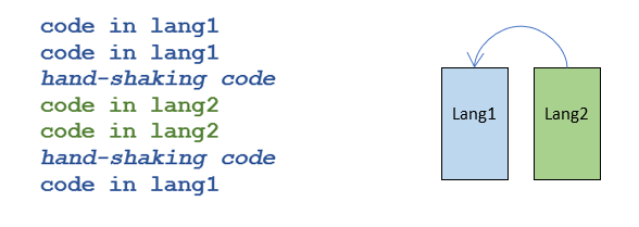
To consume a piece of code written in Python or R from within SAS, this is the only viable approach. In fact, SAS the company developed at least seven different ways of bringing open source software (OSS) into the SAS world. See the “Appendix A: OSS => SAS Integration” section later for details.
Language Level Native Integration
The “Lang2 binding” of a library written in Lang1 is a wrapper library written in Lang2 which surfaces the library’s API in syntax that are native to Lang2, so that a library written for one language can be used in another language natively.
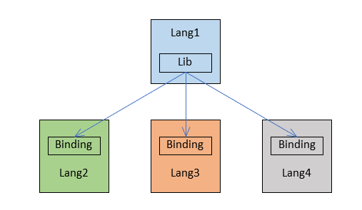
This is the preferred approach to bridge two languages and examples are abundant: H2O’s main algorithms are written with Java (!?) but it has bindings for Python, R and Scala. SAS Viya CAS actions are written with C/C++ and they provide Python, R, Lua bindings…
Data Level Hybrid Integration
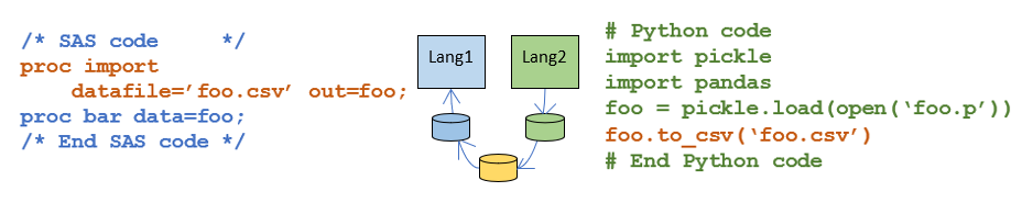
Rather than calling a different language directly, a more modular way of consuming analytical functionalities implemented in another language is reading in the result data set produced by the other language. If the host language doesn’t understand the format of the foreign data set, additional data conversion steps need to be carried out, possibly in both languages.
In below example, a pickle data frame foo produced by Python must be exported into CSV then imported into SAS before it can be consumed by SAS program.
Data Level Native Integration
When a language is equipped with data readers for data produced in other languages, the data set in foreign formats appears to be native for the host language.
Since Python and R can read SAS data set, it’s only logical for SAS to return the favor with libname engines for popular Python and R data formats such as pickled data frames, RDS or RDATA.
# SAS
libname py engine=pickle path=’C:\PyData’;
proc means data = py.foo;
GUI Level Native Integration
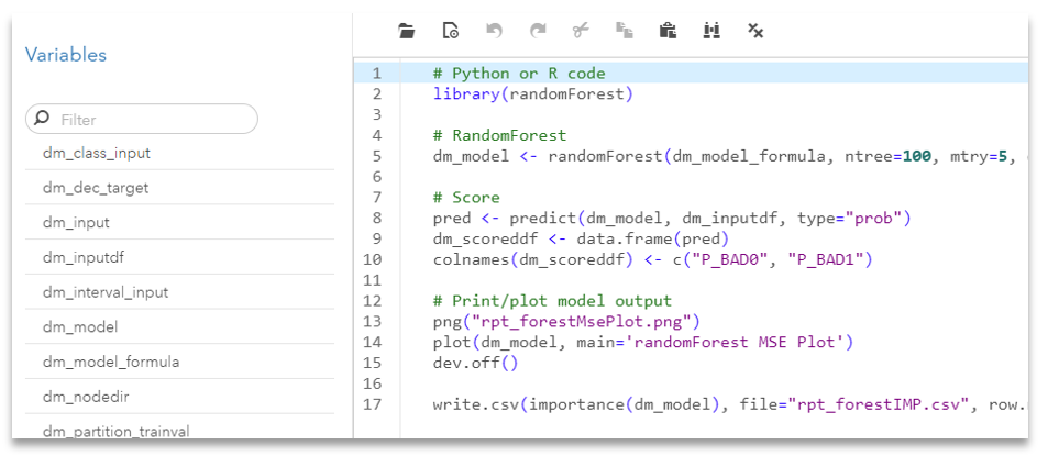
At GUI level, the ugly hand-shaking code of the hybrid approaches can be hidden from user. As shown below in SAS Viya Model Studio open source code node, users write pure Python code, without knowing that code is actually saved in a file and submitted for execution through a combination of SAS data step and Java code. The hand-shaking code is automated on user’s behalf.
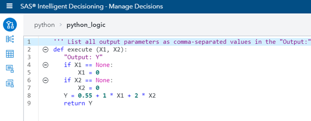
As another example of GUI level OSS integration, you may type Python code directly in a decision node and submit it for execution, without knowing the involvement of PyMAS. Bogdan Teleuca blogged about how to use Python inside a SAS Decision.
Since I currently work in a SAS shop, I don’t have much exposure to other commercial visual point-n-click analytic applications. But I’m sure there is a “code node” in each of them where you can happily type away custom code to implement the functionality not offered off the shelf.
Appendix A: Open Source Software(OSS) => SAS Integration
Unfortunately, all available routes of integration from OSS to SAS must go through at least one of its proprietary languages. In one piece of the work I did, I found myself inadvertently mixed four different languages (Data Step, CASL, FCMP, Python) in one program! Hybrid it is : (
Rants aside, if you find yourself in the situation of needing to make use of a piece of Python or R code in SAS, here are seven of your choices. I’m not surprised but please let me know if I missed any!
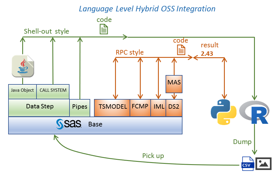
In what I call the “Shell-out” style integration, OSS code is shipped out of the SAS process for execution. Outputs of the OSS code is dumped to disk and picked up by SAS process or solution which initiates the execution. The OSS code must be written and edited in an editor outside of SAS. This style is suited when the OSS outputs are not just one or an array of numbers. Most of the GUI level integration such as the open source code node in SAS Viya Model Studio relies on this “shell-out” integration behind the scene.
In the RPC-style integration, you assemble your OSS code line by line from within one of the SAS procs. The input and outputs of your OSS code lives within the context of the hosting SAS proc. The SAS proc is responsible to send your OSS code for execution and retrieve the results back into the context of the proc. This style is suited for cases where the OSS code logic is complex, but the result is simple.
Data step > CALL SYSTEM Routine
CALL SYSTEM Routine submits an operating environment command for execution. If you strip away the SAS specific syntax such as “data _null_” and “call system” in below code, you’re as if submitting commands in an operation system shell.
data _null_;
  call system('C:\Python37\python.exe c:\ossi\hist.py');
run;
Data step > Java Object component
For those who develop solutions within the confines of the Java ecosystem, there is an unofficial SASJavaExec class, which is the Java equivalent of SAS “CALL SYSTEM” routine. The SASJavaExec class takes as parameters an executable and the code file to execute. The “executeProcess” method of the SASJavaExec data step object initiates the execution of the code file.
data _null_;
  length rtn_val 8;
  declare javaobj j("dev.SASJavaExec",        /* The class      */
                    "C:\Python37\python.exe", /* The executable */
                    "C:\ossi\hist.py");       /* The code file  */
  j.callIntMethod("executeProcess", rtn_val);
run;
This method requires knowledge of compiling java code and modifying SAS’s configuration, as described in this paper.
Base SAS pipes
A pipe is an operating system facility to pump one program’s output to another program’s input. Base SAS exposes unnamed pipe as a device type for a fileref.
filename fn pipe 'C:\Python37\python.exe C:\ossi\hist.py';

data _null_;
  infile fn;
  input;
  put _infile_;
run;
The nice thing is, any console output s from the Python program are routed to and displayed in SAS log. This is a big improvement in terms of interactivity compared with the CALL SYSTEM and Java object approaches. One fellow customer, frustrated with our lack of support to use R in SAS, built a fully interactive open source software integration experience around pipes. You edit R/Python code inside SAS editor, execute and see their outputs right in SAS’s log and results window!
The “proc_r” macro solicits the open source code from user which is wrapped around by a cards4 statement. The “run_R” macro then executes the code, displays all images produced by the code and coverts R dataset to SAS data set as requested.
%include "C:\ossi\Proc_R.sas";

%Proc_R(SAS2R=,R2SAS=);
cards4;

### R code
setwd("c:/ossi/Proc_R_Test")

C <- complex( real=rep(seq(-1.8,0.6, length.out=m), each=m ),
              imag=rep(seq(-1.2,1.2, length.out=m), m ) )
C <- matrix(C,m,m)
Z <- 0                   # initialize Z to zero
X <- array(0, c(m,m,20)) # initialize output 3D array
for (k in 1:20) {        # loop with 20 iterations
  Z <- Z^2+C             # the central difference equation
  X[,,k] <- exp(-abs(Z)) # capture results
}
write.gif(X, "Mandelbrot.gif", col=jet.colors, delay=100)
### End R code

;;;;
%run_R;
While adapting the “PROC_R” macro into my own “PROC_Py”, I had trouble displaying images… It’s time for SAS to provide official PROC R and PROC PYTHON so me and many of my colleagues don’t have to waste time on similar efforts!
PROC TSMODEL
Recently open source code support has been added within PROC TSMODEL. In below example, you declare a Python object, built up Python code line by line, run the code all from within proc TSMODEL.
PROC TSMODEL DATA=sascas1.air OUTARRAY=sascas1.outarray OUTSCALAR=sascas1.outscalar OUTOBJ=(log=sascas1.extlog);
ID date INTERVAL=MONTH;
VAR air;
OUTSCALAR runtime;
OUTARRAY pyair;
REQUIRE extlang;
SUBMIT;
    /* Copy input variable AIR into PYAIR */
    do i=1 to _LENGTH_;
        pyair[i] = air[i];
    end;

    /* Run the Python interpreter */
    declare object py(PYTHON2);
    rc = py.Initialize();
    rc = py.PushCodeLine('AIR *= 10');
    rc = py.AddVariable(pyair,'ALIAS','air','READONLY','FALSE');
    rc = py.Run();
    runtime = py.GetRuntime();

    /* Store the execution and resource usage statistics logs */
    declare object log(OUTEXTLOG);
    rc = log.Collect(py,'ALL');
ENDSUBMIT;
RUN;
Behind the scene, the External Languages Package (“package” being a special artifiact limited to the TSMODEL procedure) provides objects that enable seamless integration of external-language programs into TSMODEL procedure.
PROC FCMP
As detailed in his blog, Mike Zizzi shows how to program Python code from within PROC FCMP.
proc fcmp;
/* Declare Python object */
declare object py(python);

/* Create an embedded Python block to write your Python function */
submit into py;
def MyPythonFunction(arg1, arg2):
	"Output: ResultKey"
	Python_Out = arg1 * arg2
	return Python_Out
endsubmit;

/* Publish the code to the Python interpreter */
rc = py.publish();

/* Call the Python function from SAS */
rc = py.call("MyPythonFunction", 5, 10);

/* Store the result in a SAS variable and examine the value */
SAS_Out = py.results["ResultKey"];
put SAS_Out=;
run;
PROC IML
PROC IML provides integration from R. To get R integration, SAS must be started with the RLANG system option. Calling R functions from within proc IML is well documented. To give you a feel, in below example, R code is wrapped around proc IML “submit/R” statements. The output of the R print() function is routed to SAS results window.
proc iml;
  submit / R;
    rx <- matrix( 1:3, nrow=1)
    rm <- matrix( 1:9, nrow=3, byrow=TRUE)
    rq <- rm %*% t(rx)
    print(rq)
  endsubmit;
quit;
PROC DS2 > MAS
SAS Micro Analytic Service (MAS) is a memory-resident, high-performance program execution service. DS2 modules, running in SAS Micro Analytic Service, can publish and execute Python modules. As you can see from below example, you must build up your Python program line-by-line!
data tstinput;
    a = 8; b = 4; output;
    a = 10; b = 2; output;
run;
proc ds2;
  data _null_;
    dcl package pymas py;
    dcl int rc revision;
    dcl double a b c d;

    method init();
      dcl varchar(256) character set utf8 pycode;
      py = _new_ pymas();
      rc = py.appendSrcLine('import math');
      rc = py.appendSrcLine('# Private function example:');
      rc = py.appendSrcLine('def privfunc(x, y):');
      rc = py.appendSrcLine(' return math.hypot(x,y), math.atan2(x,y)');
      rc = py.appendSrcLine('');
      rc = py.appendSrcLine('# Public function example:');
      rc = py.appendSrcLine('def pubfunc(m, n):');
      rc = py.appendSrcLine('  "Output: o, p"');
      rc = py.appendSrcLine('  return privfunc( m, n )');
      pycode = py.getSource();
      revision = py.publish( pycode, 'ExampleModule' );
      rc = py.useMethod( 'pubfunc' );
    end;

    method run();
      set tstinput;
      rc = py.setDouble( 'm', a );
      rc = py.setDouble( 'n', b );
      rc = py.execute();
      c  = py.getDouble( 'o' );
      d  = py.getDouble( 'p' );
      put c= d=;
    end;
  enddata;
  run;
quit;
CAS => OSS Integration
Python-SWAT and R-SWAT are CAS’s Python and R bindings respectively. Regardless of the hosting language, the workflow is the same. You create a CAS session then use it as a handle to access all CAS functionalies: load action set, run actions…
import swat

# Create an CAS session
cas = swat.CAS(host, port, userid, password)
cas.loadactionset('percentile')

# Execute CAS actions
tbl  = cas.read_csv('https://raw.githubusercontent.com/'
           'sassoftware/sas-viya-programming/master/data/cars.csv')
out1 = cas.summary(table=tbl)
out2 = cas.percentile(table=tbl)

cas.close()
SAS => Python Integration
Saspy is a Python binding of SAS. When you call the means() function on the cars object, the call is translated to “proc means data=cars; run;” If you’re not used to the Pythonian way of programming, you can always drop back to the SAS way inside a sas.submit() call.
import saspy
sas  = saspy.SASsession(results='HTML')
cars = sas.sasdata('cars', libref='sashelp')
/* The MEANS procedure */
cars.means()

ll = sas.submit('''
data mycars; set sashelp.cars; myMSRP=0.001*MSRP;run;
''')
mycars = sas.sasdata('mycars', results='text')
mycars.head()
References
- More product specific OSS integration are available at GitHub.
- Amgen’s integration approach: proc groovy + Microsoft DeployR + R
- Matlab “provides a flexible, two-way integration with many programming languages, including Python. This allows different teams to work together and use MATLAB algorithms within production software and IT systems.”
- A SAS and Python double user compiles a list of resources integrate the two.
- A user’s experience of using Saspy. Another user’s instruction configuring Python and SASPy.